
SPC monitoring of characteristics by Attribute [1/2]
Attribute-based inspection is used whenever a part cannot be characterised by a number or a dimension. The result of the control will therefore be a status (good / not good) and not a measurement.
Examples of status: good / not good, beautiful / not beautiful, pass / not pass.
One may want to track the number of conforming or non-conforming products (defect tracking), or track the number of defects present on a part or in a batch of parts (defect tracking).
If we take the case of a visual inspection of the appearance of a lacquered part, we will conclude « my part is scratched or not » in the case of non-conforming products, or « my part has 0, 1, 2 or n scratches » in the case of non-conformities.
The types of statistical monitoring (calculations, limits,…) will be different for these 2 cases, and give rise to 2 types of SPC control charts in the SPC literature:
- NP cards for non-conforming (case 1 / defective products)
- C cards for non-conformities (case 2 / number of defects on a part or batch of parts)
The limitations of this monitoring
At the statistical level, attribute maps are much less relevant than measurement maps. To compensate for this lack of significance, one must work on large samples (several tens or hundreds of pieces).
We are therefore faced with new problems:
- it is not always easy to check samples with always the same (large) number of pieces (100 requested, but sometimes only 80, sometimes 112,…)
- trends and deviations are only revealed after a certain number of points, so it takes a long time (and a very large number of pieces) to get results
To answer the first problem, we can use a variant of the NP and C cards which will work in proportion (percentage of defective on a batch or of defects on a part or a batch). The calculations are obviously slightly different, but the principle remains the same.
| Follow-up of Defects | Defect Tracking | |
|---|---|---|
| In numbers | NP card | C card |
| In proportion (*) | P card | U card |
| Statistical law | Binomial Law | Poisson’s law |
(*) to remain statistically homogeneous, for proportional maps, it is considered that the sample sizes should not vary by more than 25% from a reference size.
The closer you get to zero, the better you are. And the further away you get, the more problems you have to solve.
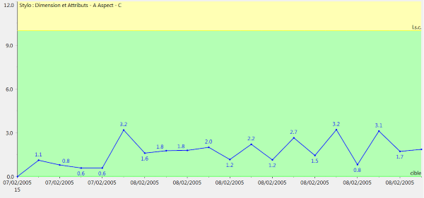
Depending on the batch sizes and the « usual » and « historical » number of defects, control limits will be calculated, and alarms will classically be triggered when these limits are exceeded.
So you can have a non-zero lower control limit! If you exceed this lower limit, you get fewer defects than « normally » (or usually…).
The same questions arise as for conventional SPC cards:
- my manufacturing process has improved! Why? How did it work? (*)
- my control process no longer works properly and no longer detects defects
(*) if my process improves, but I don’t notice it or don’t know why, it may well deteriorate again tomorrow without me knowing anything about it either !
Defect typology
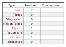
One can try to add information and meaning to these attributes, using a defect typology. If we follow a « Visual appearance » characteristic, we can make an abrupt decision as to whether or not we conform. But if we can specify why we are not in conformity, the subsequent analysis will be more precise: presence of stain ? scratch ? hole ? burr ? oxidation ?
Variants between product (NP/P) or defect (C/U) cards can always be used :
- follow-up of the defective ones: non-conforming aspect because of the presence of holes and scratches
- follow-up of the defects: non-conforming aspect as there are 2 holes and 3 scratches !
We can also add a weight (or a cost) to our types of defects: some are more serious or critical than others (statistically speaking, we can then speak of a « D » card, a demerit card). The point followed on the control chart will be calculated according to the weight of each type of defect, and if the weight is important, we will reach the control limit « faster »: we will be alerted !
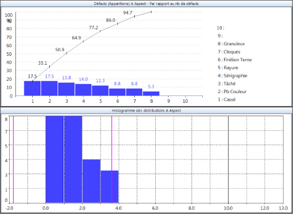
The other advantage of following an attribute map with a fault typology is that it allows an analysis with a pareto diagram:
- pareto of occurrence of defects (weighted or not)
- calculated as a % of the number of parts (or the number of defects)
General issue
The problem associated with this type of control is linked to the very nature of the attribute: it is not very meaningful (good, not good…).
To improve what can be learned from it, we work in two directions:
- the number of parts to be checked (the sample size): we try to work on a large number of parts, which is not always easy, not always possible, and which takes a lot of time!
- the characterisation of defects: we try to add a type to the defects, or a class. This brings us to another problem, which is the « measurement » of the defect. Attributive controls are mostly manual! And one controller may have a different opinion or status from his colleague. R&R studies related to attribute characteristics sometimes hold surprises…
Even further
If we want to go even further, we can use the notion of Defect Map, or defect mapping. Indeed, the same defect will not have the same importance or the same criticality depending on its location!
Example: I check flat glass for conservatory windows.
A scratch is a defect, which I must follow. I must be alerted to the presence of scratches.
But a scratch in the middle of the pane is critical (discarded part) while the same scratch on the periphery is acceptable (hidden by the window posts).
It is therefore necessary to add a « location » parameter to the defect, or even « dimensional » characteristics: large scratch? small scratch?
This will be the focus of our next blog post on the Defect Map!
Frédéric Henrionnet
Quality Assurance Manager, Infodream
Read also: Defect Map – an attributive control introducing the notion of fault location (2/2)
Learn more about Qual@xy SPC
Learn more about Defect Map